Vibrational analysis

Vibrational analysis#

The vibrational analysis interface simply leverages the job parallelization feature of the MatSciToolkit so we have a more reliable (less chance of failure) and faster calculation.

Note

Compatability

Currently, only Quantum Espresso is supported. The code is still in development and will be expanded to other codes in the future (as needed).

Example files#

A set of example files are provided in the tutorial folder of the MatSciToolkit repository. Specifically, the vibrational analysis calculation is demonstrated in the example_ase_vib_1 directory.

Example files workflow#

The workflow in the example is as follows:

(01 prefix) Generate the displaced structures with ID
(02 prefix) Distribute and run the displaced structures in parallel.
(03 prefix) Combine the results and save as ASE readable cache
(04 prefix) Post-process the data and plot the results

Workflow parts#

Job distributed parallelization#

In this vibrational analysis case, we don’t need to discuss the dipole moment yet so let’s focus on the job distributed parallelization.

After the 01_generate_displaced_structures.py was run, you will end up with a set of displaced structures in .vasp format. You will need to count how many it is and assign the Job array range based on that. In the example, you will get 25 displaced structures (starting with 1 to 25), hence the job array should be 1-25. The corresponding job submission script should look like this:

#!/bin/bash
#$ -S /bin/bash
#$ -cwd
#$ -q xs2.q
#$ -pe x16 16
#$ -j y
#$ -N calc_02_dftrun
#$ -t 1-25          # Job array range

python 02_run_dft_calculation.py --id $SGE_TASK_ID

DFTrunner class#

Instead of calling the Espresso class, we call the DFTrunner class which is a wrapper for the Espresso class like so:

import argparse
argparser = argparse.ArgumentParser()
argparser.add_argument("-i", "--id", type=int)
args = argparser.parse_args()

x = DFTrunner(
    system_id=args.id, # JOB array id -> displaced image id
    input_data=input_data, # No need for specific parameter for dipole moment
    pseudopotentials=pseudopotentials, 
    kpts=[12, 12, 1],
    dirname="dft_calc/SUFFIX",
    espresso_command="mpirun pw.x".split(),
)

We just input the ID and get the displaced structure based on that. The DFTrunner will run the DFT calculation and print out the necessary data that can be used for ASE’s vibrational analysis.

This is quite simple and technically, you can code this in python, however, the MatSciToolkit provides a wrapper for this to make it easier.

Collector#

After all the DFT calculations are done, we need to collect the data and save it as an ASE readable cache. This is done by the 03_collector.py script.

Post-processing#

In post-processing, we try to output all the necessary plots and files. The implementation is parallelized (with python’s multiprocessing) because making the GIFs for each mode can be quite slow (especially if you have a lot of modes).

x = PostProcess(nproc=16)
x.generate_summary()
x.generate_spectra()
x.load_summary()
x.load_spectra()
x.generate_mode_traj()
x.generate_mode_gif()
x.generate_spectra_plot()

Example outputs#

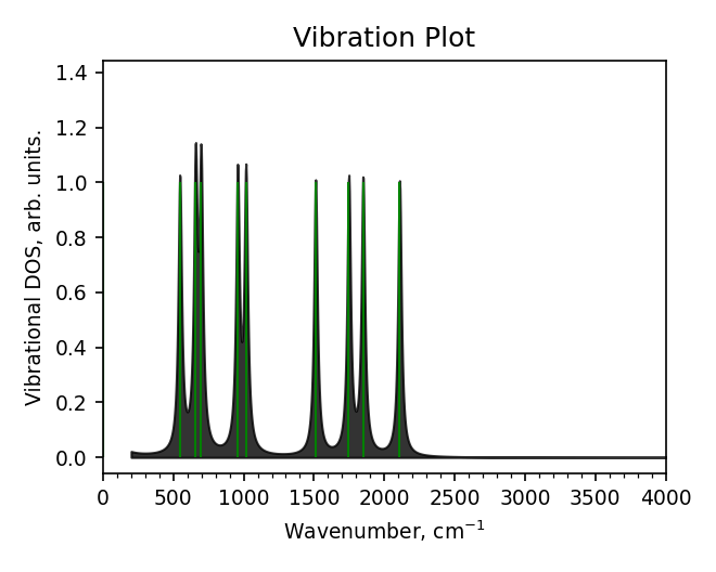
Spectra#

Spectra data file (report_spectra.dat)#

# Lorentzian folded, width=30 cm^-1
# [cm^-1] arbitrary
000      2.18012e-02
000      2.13743e-02
000      2.09700e-02
000      2.05872e-02
000      2.02249e-02
000      1.98821e-02
000      1.95577e-02
000      1.92510e-02
000      1.89612e-02
000      1.86876e-02
000      1.84294e-02
000      1.81861e-02
...
...

Spectra plot (report_spectra.png)#

Vibrational mode#

Trajectory file#

user@user:~$ ls vib_modes/*traj
vib_modes/vib.0.traj   vib_modes/vib.11.traj  vib_modes/vib.4.traj  vib_modes/vib.7.traj
vib_modes/vib.1.traj   vib_modes/vib.2.traj   vib_modes/vib.5.traj  vib_modes/vib.8.traj
vib_modes/vib.10.traj  vib_modes/vib.3.traj   vib_modes/vib.6.traj  vib_modes/vib.9.traj

GIFs#