Infrared analysis

Infrared analysis#

The infrared analysis interface is more complex than the vibrational analysis. It combines the job parallelization, dipole moment calculation and a multi-directional dipole moment combiner. The good thing is MatSciToolkit handles all of these for you.

Note

Compatability

Currently, only Quantum Espresso is supported. The code is still in development and will be expanded to other codes in the future (as needed).

Example files#

A set of example files are provided in the tutorial folder of the MatSciToolkit repository. Specifically, the infrared analysis calculation is demonstrated in the example_ase_ir_1 directory.

Example files workflow#

The workflow in the example is as follows:

(01 prefix) Generate the displaced structures with ID
(02 prefix) Distribute and run the displaced structures in parallel.
(03 prefix) Combine the results and save as ASE readable cache
(04 prefix) Post-process the data and plot the results

Important parts in the input_data for DFT runs#

Instead of calling the Espresso class, we call the DFTrunner class which is a wrapper for the Espresso class like so:

# Not the full code, please check the example files for the full code
import argparse
argparser = argparse.ArgumentParser()
argparser.add_argument("-i", "--id", type=int)
args = argparser.parse_args()

x = DFTrunner(
    system_id=args.id,
    input_data=input_data,
    pseudopotentials=pseudopotentials,
    kpts=[12, 12, 1],
    dirname="dft_calc/SUFFIX",
    espresso_command="mpirun pw.x".split(),
    field_directions=[3],
    emaxpos="auto",
    eamp=0.0,
    eopreg=0.0001,
)

Here, we pass the Job array ID ($SGE_TASK ID in PBS system) to get the displaced structure and run it with the DFT runner.

Unlike in the dipole moment calculation where we needed to put specific parameters for the electric field. In this workflow, the code handles it for us so we only need to put the standard DFT parameters. This is handled this way because in multi-directional systems (say, 2D or 1D systems), we need to calculate the dipole moment in all directions (which means 2 or 3 dft runs per displaced structure) and combine them.

Just for the sake of completeness, the emaxpos, eamp, eopreg values are assign a value, however, this is also the default value so you can remove it if you want. emaxpos=auto just means we allow the workflow to check by itself the farthest point. The important parameter here is the field_directions which is a list of directions you want to calculate the dipole moment for (1=x, 2=y, 3=z). Here we set field_directions=[3] because our system is a two-dimensional sheet, hence, we only need to calculate the dipole moment in the z-direction.

Workflow parts#

Most parts are similar to the vibrational analysis. There is only a slight difference with the dipole_collector since we are now collecting the dipole moment in multiple direction as well.

Example outputs#

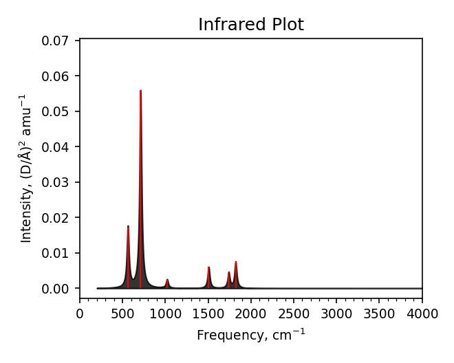
Spectra summary#

-------------------------------------
 Mode    Frequency        Intensity
  #    meV     cm^-1   (D/Å)^2 amu^-1
-------------------------------------
  0    0.2i      1.4i     0.0006
  1    0.1i      0.8i     0.0000
  2    0.0i      0.1i     0.0000
  3   69.7     562.1      0.0172
  4   81.1     654.3      0.0001
  5   88.1     710.2      0.0558
  6  119.0     959.8      0.0001
  7  126.5    1020.3      0.0024
  8  186.8    1506.4      0.0060
  9  215.8    1740.4      0.0044
 10  225.8    1821.2      0.0075
 11  259.4    2092.0      0.0000
-------------------------------------
Zero-point energy: 0.686 eV
Static dipole moment: 0.005 D
Maximum force on atom in `equilibrium`: 0.1036 eV/Å

Spectra data#

# Lorentzian folded, width=30 cm^-1
# [cm^-1] [(D/Å)^2 amu^-1]
000      8.38984e-05      9.98501e-01 
000      8.48792e-05      9.98484e-01 
000      8.58872e-05      9.98466e-01 
000      8.69228e-05      9.98447e-01 
000      8.79864e-05      9.98428e-01 
000      8.90786e-05      9.98409e-01 
000      9.02000e-05      9.98389e-01 
000      9.13511e-05      9.98368e-01 
000      9.25326e-05      9.98347e-01 
000      9.37452e-05      9.98325e-01 
000      9.49895e-05      9.98303e-01 
...
...

Spectra plot#

Spectra modes (trajectory file)#

user@user:~$ ls ir_modes/*traj
ir_modes/ir.0.traj   ir_modes/ir.4.traj
ir_modes/ir.1.traj   ir_modes/ir.5.traj
ir_modes/ir.10.traj  ir_modes/ir.6.traj
ir_modes/ir.11.traj  ir_modes/ir.7.traj
ir_modes/ir.2.traj   ir_modes/ir.8.traj
ir_modes/ir.3.traj   ir_modes/ir.9.traj

Spectra GIF#